Análisis Factorial Exploratorio II
0. Objetivo del práctico
El objetivo de este práctico revisar como realizar un Análisis factorial Exploratorio en R considerando la selección del número de factores, la extracción de factores, la rotación, la selección del modelo final y su interpretación, y el cálculo de puntuaciones factoriales. Este en una continuación del práctico anterior, donde realziamos la gestión de datos y la comprobación de los supuestos del análisis.
1. Carga y gestión de datos y librerias
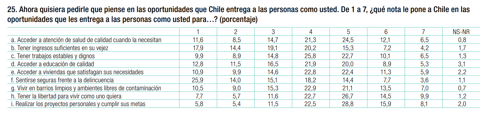
Cargamos nuevamente la base de datos de PNUD 2015, que incluye los siguientes ítem. Con estos esperamos revisar si existen estructuras latentes en como las personas evalúan las oportunidades que entrega Chile. Además eliminamos los casos perdidos y atípicos. Para los detalles estas decisiones, revisar el práctico anterior.
datosog <- read.csv("https://raw.githubusercontent.com/Clases-GabrielSotomayor/pruebapagina/master/static/slides/data/EDH_2013_csv.csv")

datos<-datosog[,c("cor","P25a","P25b","P25c","P25d","P25e","P25f","P25g","P25h","P25i")]

#Codificar perdidos como NA
datos[datos==9] <- NA
datos[datos==8] <- NA
#Eliminar perdidos
datosLW <- na.omit(datos)
#Tratamiento de casos atipicos
mean<-colMeans(datosLW[1:9])
Sx<-cov(datosLW[1:9]) #matriz de varianza covariaza
D2<-mahalanobis(datosLW[1:9],mean,Sx)
datosLW$sigmahala=(1-pchisq(D2, 3))
datosLW<-datosLW[which(datosLW$sigmahala>0.001),]#dar por perdido o eliminar caso atipico
datosLW$sigmahala<-NULL

#guardar id para hacer el merge luego con otras variables
id<-datosLW$cor
datosLW$cor<-NULL

colnames(datosLW)<-c("SALUD" ,"INGR" , "TRAB",  "EDUC"  ,"VIVI" , "SEGUR","MEDIO" ,"LIBER" ,"PROYE")
Cargamos el paquete “psych” que nos permitirá realizar en análisis factorial exporatorio (AFE), “GPArotation” para poder hacer rotación promax, y “dplyr()” para gestión de datos.
library(psych)
library(GPArotation)
library(dplyr)
2. Análisis factorial exploratorio
Gráfico de sedimentación
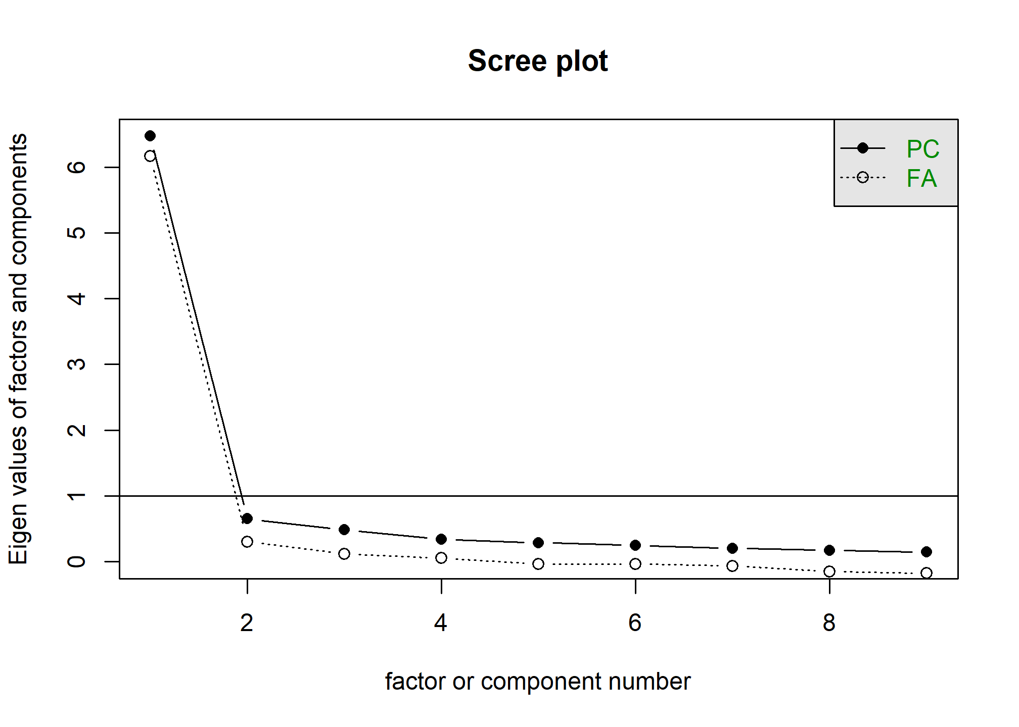
El gráfico de sedimentación (scree plot) nos ayuda a decidir cuántos factores mantener en el análisis. Para ello, utilizaremos la función scree() de la librería psych.
El gráfico de sedimentación muestra la proporción de varianza explicada por cada factor en el eje Y y el número de factores en el eje X. Se busca identificar un punto de inflexión en la gráfica, donde la pendiente de la curva se aplana. Este punto indica la cantidad de factores que se deben retener.
scree(datosLW)
Selección del número de factores
Para decidir cuántos factores incluir en el análisis factorial, utilizaremos la función fa.parallel() de la librería psych. Esta función utiliza análisis paralelos para determinar cuántos factores se deben retener.
nofactor <- fa.parallel(datosLW, fa="fa")
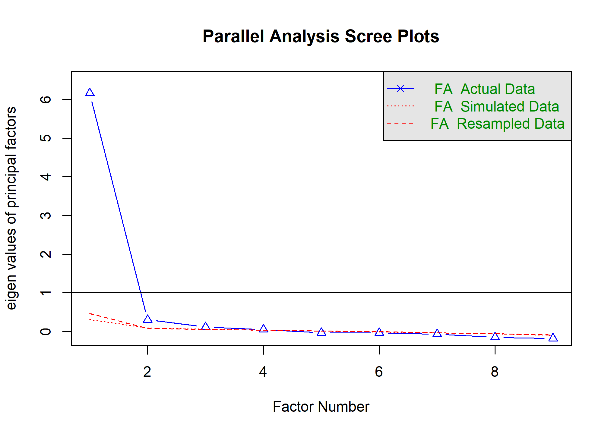
## Parallel analysis suggests that the number of factors = 3 and the number of components = NA
nofactor$fa.values
## [1]  6.16459264  0.30104369  0.11682746  0.05037410 -0.03516097 -0.03677260
## [7] -0.06750294 -0.15161530 -0.17719329
En este caso, el análisis paralelo sugiere retener 4 factores.
Análisis factorial exploratorio con diferentes configuraciones
Ahora realizaremos el análisis factorial exploratorio utilizando diferentes configuraciones, como el número de factores, rotaciones y correlaciones. Esto nos permitirá comparar y seleccionar el mejor modelo.
Cuando se trabaja con variables ordinales o categóricas en un análisis factorial exploratorio, es más apropiado utilizar correlaciones policóricas, ya que tienen en cuenta la naturaleza no lineal y discreta de los datos. Dado que nuestras variables tienen 7 categorías probamos ambos tipos de correlaciones para ver el nivel de ajuste. El análisis con correlaciones policóricas explica una mayor proporción de la varianza por lo que se seguirá con estas.
# Prueba de Modelos segun parallel
fa(datosLW,nfactors=4, fm="minres",rotate="none")
## Factor Analysis using method =  minres
## Call: fa(r = datosLW, nfactors = 4, rotate = "none", fm = "minres")
## Standardized loadings (pattern matrix) based upon correlation matrix
##        MR1   MR2   MR3   MR4   h2     u2 com
## SALUD 0.80  0.12 -0.08 -0.02 0.66 0.3441 1.1
## INGR  0.84  0.44 -0.14  0.27 1.00 0.0045 1.8
## TRAB  0.86  0.01 -0.17 -0.14 0.78 0.2168 1.1
## EDUC  0.89  0.06 -0.03 -0.20 0.83 0.1655 1.1
## VIVI  0.88  0.02  0.04 -0.18 0.81 0.1865 1.1
## SEGUR 0.74  0.21  0.35  0.01 0.72 0.2794 1.6
## MEDIO 0.82 -0.14  0.18  0.07 0.73 0.2742 1.2
## LIBER 0.87 -0.45  0.00  0.20 1.00 0.0037 1.6
## PROYE 0.82 -0.24 -0.11  0.01 0.74 0.2629 1.2
##
##                        MR1  MR2  MR3  MR4
## SS loadings           6.28 0.54 0.23 0.21
## Proportion Var        0.70 0.06 0.03 0.02
## Cumulative Var        0.70 0.76 0.78 0.81
## Proportion Explained  0.87 0.07 0.03 0.03
## Cumulative Proportion 0.87 0.94 0.97 1.00
##
## Mean item complexity =  1.3
## Test of the hypothesis that 4 factors are sufficient.
##
## The degrees of freedom for the null model are  36  and the objective function was  8.31 with Chi Square of  12155.21
## The degrees of freedom for the model are 6  and the objective function was  0.02
##
## The root mean square of the residuals (RMSR) is  0.01
## The df corrected root mean square of the residuals is  0.01
##
## The harmonic number of observations is  1467 with the empirical chi square  2.82  with prob <  0.83
## The total number of observations was  1467  with Likelihood Chi Square =  30.64  with prob <  3e-05
##
## Tucker Lewis Index of factoring reliability =  0.988
## RMSEA index =  0.053  and the 90 % confidence intervals are  0.035 0.072
## BIC =  -13.11
## Fit based upon off diagonal values = 1
## Measures of factor score adequacy
##                                                    MR1  MR2   MR3  MR4
## Correlation of (regression) scores with factors   0.99 0.99  0.70 0.87
## Multiple R square of scores with factors          0.98 0.98  0.50 0.76
## Minimum correlation of possible factor scores     0.96 0.96 -0.01 0.52
# Prueba con 4 factores y correlación polychoric
fa(datosLW, nfactors=4, rotate="none", cor = "poly")
## Factor Analysis using method =  minres
## Call: fa(r = datosLW, nfactors = 4, rotate = "none", cor = "poly")
## Standardized loadings (pattern matrix) based upon correlation matrix
##        MR1   MR2   MR3   MR4   h2     u2 com
## SALUD 0.81  0.13 -0.10  0.00 0.68 0.3188 1.1
## INGR  0.86  0.42 -0.11  0.27 1.00 0.0046 1.7
## TRAB  0.87  0.01 -0.19 -0.11 0.81 0.1907 1.1
## EDUC  0.91  0.06 -0.06 -0.19 0.87 0.1335 1.1
## VIVI  0.90  0.03  0.02 -0.19 0.84 0.1565 1.1
## SEGUR 0.78  0.21  0.36 -0.03 0.78 0.2187 1.6
## MEDIO 0.84 -0.15  0.19  0.05 0.76 0.2368 1.2
## LIBER 0.88 -0.44  0.02  0.17 1.00 0.0026 1.6
## PROYE 0.84 -0.25 -0.10  0.02 0.78 0.2249 1.2
##
##                        MR1  MR2  MR3  MR4
## SS loadings           6.57 0.52 0.24 0.19
## Proportion Var        0.73 0.06 0.03 0.02
## Cumulative Var        0.73 0.79 0.81 0.83
## Proportion Explained  0.87 0.07 0.03 0.03
## Cumulative Proportion 0.87 0.94 0.97 1.00
##
## Mean item complexity =  1.3
## Test of the hypothesis that 4 factors are sufficient.
##
## The degrees of freedom for the null model are  36  and the objective function was  9.37 with Chi Square of  13698.35
## The degrees of freedom for the model are 6  and the objective function was  0.03
##
## The root mean square of the residuals (RMSR) is  0.01
## The df corrected root mean square of the residuals is  0.01
##
## The harmonic number of observations is  1467 with the empirical chi square  2.72  with prob <  0.84
## The total number of observations was  1467  with Likelihood Chi Square =  38.74  with prob <  8.1e-07
##
## Tucker Lewis Index of factoring reliability =  0.986
## RMSEA index =  0.061  and the 90 % confidence intervals are  0.044 0.08
## BIC =  -5.01
## Fit based upon off diagonal values = 1
## Measures of factor score adequacy
##                                                    MR1  MR2  MR3  MR4
## Correlation of (regression) scores with factors   0.99 0.99 0.74 0.88
## Multiple R square of scores with factors          0.99 0.98 0.54 0.78
## Minimum correlation of possible factor scores     0.97 0.96 0.09 0.56
La rotación de factores es un paso importante en el AFE, ya que facilita la interpretación de los resultados. La rotación puede ser ortogonal o oblicua. La rotación ortogonal (e.g. varimax) asume que los factores no están correlacionados, mientras que la rotación oblicua (e.g. promax) permite que los factores estén correlacionados.
Para decidir qué rotación utilizar, es útil explorar la correlación entre los factores. Si las correlaciones son bajas (menores a 0.3), la rotación ortogonal es apropiada. Si las correlaciones son altas, se recomienda utilizar la rotación oblicua.
# Prueba con 3 factores y rotación varimax y promax
fa(datosLW, nfactors=4, rotate="varimax", cor = "poly")
## Factor Analysis using method =  minres
## Call: fa(r = datosLW, nfactors = 4, rotate = "varimax", cor = "poly")
## Standardized loadings (pattern matrix) based upon correlation matrix
##        MR2  MR1  MR4  MR3   h2     u2 com
## SALUD 0.37 0.47 0.48 0.30 0.68 0.3188 3.6
## INGR  0.27 0.33 0.83 0.35 1.00 0.0046 1.9
## TRAB  0.46 0.62 0.40 0.24 0.81 0.1907 3.0
## EDUC  0.42 0.64 0.36 0.38 0.87 0.1335 3.1
## VIVI  0.44 0.60 0.31 0.44 0.84 0.1565 3.4
## SEGUR 0.28 0.29 0.35 0.70 0.78 0.2187 2.2
## MEDIO 0.61 0.30 0.27 0.48 0.76 0.2368 2.8
## LIBER 0.89 0.29 0.23 0.25 1.00 0.0026 1.5
## PROYE 0.68 0.44 0.28 0.21 0.78 0.2249 2.3
##
##                        MR2  MR1  MR4  MR3
## SS loadings           2.51 1.92 1.65 1.44
## Proportion Var        0.28 0.21 0.18 0.16
## Cumulative Var        0.28 0.49 0.67 0.83
## Proportion Explained  0.33 0.26 0.22 0.19
## Cumulative Proportion 0.33 0.59 0.81 1.00
##
## Mean item complexity =  2.7
## Test of the hypothesis that 4 factors are sufficient.
##
## The degrees of freedom for the null model are  36  and the objective function was  9.37 with Chi Square of  13698.35
## The degrees of freedom for the model are 6  and the objective function was  0.03
##
## The root mean square of the residuals (RMSR) is  0.01
## The df corrected root mean square of the residuals is  0.01
##
## The harmonic number of observations is  1467 with the empirical chi square  2.72  with prob <  0.84
## The total number of observations was  1467  with Likelihood Chi Square =  38.74  with prob <  8.1e-07
##
## Tucker Lewis Index of factoring reliability =  0.986
## RMSEA index =  0.061  and the 90 % confidence intervals are  0.044 0.08
## BIC =  -5.01
## Fit based upon off diagonal values = 1
## Measures of factor score adequacy
##                                                    MR2  MR1  MR4  MR3
## Correlation of (regression) scores with factors   0.99 0.86 0.97 0.79
## Multiple R square of scores with factors          0.98 0.73 0.95 0.63
## Minimum correlation of possible factor scores     0.96 0.47 0.90 0.26
fa(datosLW, nfactors=4, rotate="promax", cor = "poly")
## Factor Analysis using method =  minres
## Call: fa(r = datosLW, nfactors = 4, rotate = "promax", cor = "poly")
## Standardized loadings (pattern matrix) based upon correlation matrix
##         MR1   MR2   MR4   MR3   h2     u2 com
## SALUD  0.45  0.09  0.31  0.05 0.68 0.3188 1.9
## INGR   0.02  0.00  0.92  0.09 1.00 0.0046 1.0
## TRAB   0.76  0.14  0.12 -0.10 0.81 0.1907 1.2
## EDUC   0.81  0.02  0.00  0.13 0.87 0.1335 1.1
## VIVI   0.71  0.07 -0.07  0.25 0.84 0.1565 1.3
## SEGUR  0.06 -0.04  0.10  0.79 0.78 0.2187 1.0
## MEDIO  0.03  0.54  0.00  0.38 0.76 0.2368 1.8
## LIBER -0.06  1.05  0.01 -0.02 1.00 0.0026 1.0
## PROYE  0.36  0.63  0.02 -0.10 0.78 0.2249 1.7
##
##                        MR1  MR2  MR4  MR3
## SS loadings           2.76 2.24 1.27 1.24
## Proportion Var        0.31 0.25 0.14 0.14
## Cumulative Var        0.31 0.56 0.70 0.83
## Proportion Explained  0.37 0.30 0.17 0.17
## Cumulative Proportion 0.37 0.67 0.83 1.00
##
##  With factor correlations of
##      MR1  MR2  MR4  MR3
## MR1 1.00 0.80 0.78 0.76
## MR2 0.80 1.00 0.62 0.69
## MR4 0.78 0.62 1.00 0.70
## MR3 0.76 0.69 0.70 1.00
##
## Mean item complexity =  1.3
## Test of the hypothesis that 4 factors are sufficient.
##
## The degrees of freedom for the null model are  36  and the objective function was  9.37 with Chi Square of  13698.35
## The degrees of freedom for the model are 6  and the objective function was  0.03
##
## The root mean square of the residuals (RMSR) is  0.01
## The df corrected root mean square of the residuals is  0.01
##
## The harmonic number of observations is  1467 with the empirical chi square  2.72  with prob <  0.84
## The total number of observations was  1467  with Likelihood Chi Square =  38.74  with prob <  8.1e-07
##
## Tucker Lewis Index of factoring reliability =  0.986
## RMSEA index =  0.061  and the 90 % confidence intervals are  0.044 0.08
## BIC =  -5.01
## Fit based upon off diagonal values = 1
## Measures of factor score adequacy
##                                                    MR1 MR2  MR4  MR3
## Correlation of (regression) scores with factors   0.97   1 1.00 0.92
## Multiple R square of scores with factors          0.94   1 0.99 0.85
## Minimum correlation of possible factor scores     0.88   1 0.99 0.71
# Modelo final
modelofinal <- fa(datosLW, nfactors=4, rotate="promax", cor = "poly")
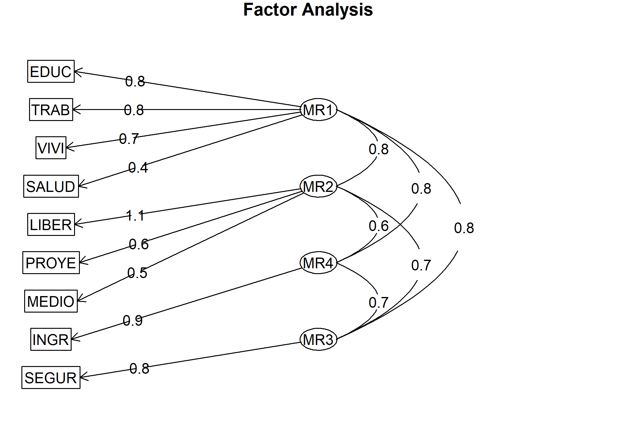
Después de comparar los resultados, decidimos utilizar un modelo con 4 factores y rotación promax.
Visualización de resultados
Podemos observar los resultados del análisis con el comando fa.diagram(), que nos muestra las cargas factoriales de los ítems del modelo con cada uno de los factores latentes.
fa.diagram(modelofinal)
Cálculo de puntuaciones factoriales
Finalmente, podemos calcular las puntuaciones factoriales para cada individuo en nuestra muestra utilizando la función factor.scores(). Estas puntuaciones pueden ser utilizadas en análisis posteriores o como variables en otros modelos
#Extracción de puntuaciones factoriales

#Extraemos las puntuaciones facotriales del objeto del modelo final
summary(modelofinal$scores)
##       MR1                MR2               MR4               MR3
##  Min.   :-1.97980   Min.   :-2.1845   Min.   :-1.5535   Min.   :-1.838369
##  1st Qu.:-0.68995   1st Qu.:-0.6839   1st Qu.:-0.8592   1st Qu.:-0.711958
##  Median : 0.05109   Median : 0.1777   Median :-0.2056   Median : 0.005353
##  Mean   : 0.00000   Mean   : 0.0000   Mean   : 0.0000   Mean   : 0.000000
##  3rd Qu.: 0.71403   3rd Qu.: 0.6565   3rd Qu.: 0.8679   3rd Qu.: 0.693281
##  Max.   : 2.06091   Max.   : 1.8364   Max.   : 2.1276   Max.   : 2.200736
#Guardamos los puntajes en la base
basefinal<-cbind(datosLW,modelofinal$scores )

#Pegamos la variable GSE de la base de datos original
datosog<-filter(datosog, datosog$cor%in% id)
basefinal<-cbind(basefinal,datosog$GSEo)
basefinal$gse<-factor(basefinal$`datosog$GSEo`,1:4,labels = c("ABC1"  , "C2" ,  "C3"  ,  "D"))

#Comparamos el
aggregate(basefinal$MR1,list(basefinal$gse),mean) #Derechos sociales
##   Group.1           x
## 1    ABC1  0.70051863
## 2      C2  0.09371833
## 3      C3 -0.12322170
## 4       D -0.12702080
aggregate(basefinal$MR2,list(basefinal$gse),mean) #Derechos individuales
##   Group.1          x
## 1    ABC1  0.6721192
## 2      C2  0.1465837
## 3      C3 -0.1287113
## 4       D -0.1370771
#aggregate(basefinal$MR3,list(basefinal$gse),mean) #Jubilación
#aggregate(basefinal$MR4,list(basefinal$gse),mean) #Seguridad